Machine Learning, ChatGPT, and Bayes’s Theorem – Part 2

The role of probability in machine learning.

This continues an essay series on how the sort of AI that entails what’s become called “machine learning” works, using Anil Ananthaswamy’s book Why Machines Learn: The Elegant Math Behind Modern AI, and Tom Chivers’ book Everything Is Predictable: How Bayesian Statistics Explain Our World, to help explain things.  This essay focuses on the role of probability in machine learning.

As Ananthaswamy writes:

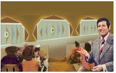
Probability deals with reasoning in the presence of uncertainty. And it’s a fraught business for the best of us. There’s no better illustration of how uncertainty messes with our minds than the Monty Hall dilemma. The problem, named after the host of the American television show Let’s Make a Deal, became a public obsession in 1990 when a reader of the Parade magazine column “Ask Marilyn” posed the following question to columnist Marilyn vos Savant: “Suppose you are on a game show, and you’re given the choice of three doors. Behind one is a car; behind the others, goats. You pick a door, say, No. 1, and the host, who knows what’s behind the doors, opens another door, say, No. 3, which has a goat. He then says to you, ‘Do you want to pick No. 2?’ Is it to your advantage to switch your choice?” The person playing the game has a quandary. Do they switch their choice from door No. 1 to door No. 2? Is there any benefit to doing so, in that they will increase their odds of choosing the door hiding the car? Before we look at vos Savant’s answer, let’s try to tackle the problem ourselves.

Here’s my intuitive answer: Before the host opens one of the doors, the probability that a car is behind the door I’ve picked (Door No. 1) is one-third. But then the host opens Door No. 3 and reveals that there’s a goat behind it. Now there are two closed doors, and behind one of them is the car. I figure that the car is equally likely to be behind one or the other door. There’s no reason to switch my choice. You may or may not have reasoned similarly. Kudos if you didn’t. Here’s what vos Savant advised regarding whether you should switch your choice: “Yes; you should switch. The first door has a one-third chance of winning, but the second door has a two-thirds chance.” And she’s correct … Vos Savant stood her ground and provided the critics with different ways of arriving at her answer. One of her best intuitive arguments, paraphrasing her, asks you to consider a different situation. Say there are a million doors, and behind one of them is a car; all the others hide goats. You choose Door No. 1. There’s a one-in-a-million chance you are correct. The host then opens all the other doors you did not choose, except one. Now there are two unopened doors, your choice and the one the host left closed. Sure, the latter door could hide a goat. But of all the doors the host chose not to open, why did he choose that one? “You’d switch to that door pretty fast, wouldn’t you?” wrote vos Savant. Mathematician Keith Devlin gave another take on it. Put a mental box around your choice, Door No. 1, and another box around Doors No. 2 and 3 combined. The box around Door No. 1 has a one-third probability associated with it, and the box around Doors No. 2 and 3 has a two-thirds probability associated with it, in terms of containing the car. Now the host opens one of the doors inside the bigger box to reveal a goat. The two-thirds probability of the bigger box shifts to the unopened door. To switch is the correct answer … Andrew Vázsonyi [later] used a computer program he had written to run one hundred thousand simulations of the game and showed that the host won and you lost two-thirds of the time if you didn’t switch, but the host lost and you won two-thirds of the time if you did switch.

Chivers uses another example to explain the logic behind the solution to the Monty Hall problem:

Assuming that Monty knows which door the car is behind, and that he always opens one of the other ones, you should switch. There are a few ways to grasp this intuitively. One is to imagine that, instead of a choice of three doors, you’d originally had a choice of 1 million doors. Once again, one of them hides a car. (And you would like a car.) You choose one. Then Monty opens 999,998 doors, showing that all of them are empty. Now you’re left with just two, your original choice and one other. But what’s crucial is that Monty, first, knows where the car is, and second, always opens a door with a goat behind it. Once that’s stipulated—or assumed—you can easily work out the odds with Bayes’ rule. At the start, your probability that the car is behind any given door is one-third, or p ≈ 0.33. You have no information that gives you any reason to pick any one over the others. But Monty, if he knows where the car is and always opens a door, gives you some information; he allows you to update your prior probabilities. It’s easier if we use odds. The odds of the car being behind Door #1, #2, or #3 are 1:1:1: that is, there’s nothing between them. That’s still true even after you pick Door #1. Then Monty opens Door #3 and reveals a goat. The probability that he’d open Door #3 if you’re right and the car is behind Door #1 is 50 percent—he could have picked either of the other doors. But if the car is behind Door #2, then it’s 100 percent certain that he’d have picked Door #3. And if it was behind Door #3, there’s a 0 percent chance. So the odds are 1:2:0. That’s your likelihood, or your Bayes factor. You might just remember that when you’re doing Bayes’ theorem with odds, it’s nice and easy: you just multiply your prior odds with your Bayes factor and you get your posterior odds. 1:1:1 times 1:2:0 is 1:2:0. You know it’s not in #3, and it’s twice as likely to be in #2 as #1. But now imagine a different scenario, where Monty doesn’t always open a wrong door, or he doesn’t always open a door at all. Or if you don’t know if Monty has any particular strategy. Imagine that Monty actually flips a coin, and if it comes up heads, he opens the lower-numbered of the two remaining doors. Or Monty’s not even doing it: an earthquake hits the TV studio just after you make your decision, and one of the two remaining doors happens to swing open. Then you’re not gaining any information about the door you picked. The prior odds are 1:1:1, but the chance that Door #2 would be the one that happened to open is fifty-fifty whether or not you picked the right one, so your likelihood odds are 1:1:0 and therefore your posterior odds are 1:1 as well. Then it really doesn’t make any difference whether you stick or twist.

Judea Pearl and Dana Mackenzie explain the paradox in this useful way in their book The Book of Why: The New Science of Cause and Effect:

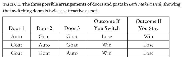
Let’s take a look first at how vos Savant solved the puzzle. Her solution is actually astounding in its simplicity and more compelling than any I have seen in many textbooks. She made a list (Table 6.1) of the three possible arrangements of doors and goats, along with the corresponding outcomes under the “Switch” strategy and the “Stay” strategy. All three cases assume that you picked Door 1. Because all three possibilities listed are (initially) equally likely, the probability of winning if you switch doors is two-thirds, and the probability of winning if you stay with Door 1 is only one-third. Notice that vos Savant’s table does not explicitly state which door was opened by the host. That information is implicitly embedded in columns 4 and 5. For example, in the second row, we kept in mind that the host must open Door 3; therefore switching will land you on Door 2, a win. Similarly, in the first row, the door opened could be either Door 2 or Door 3, but column 4 states correctly that you lose in either case if you switch … [H]ow come your belief in Door 2 has gone up from one-third to two-thirds? The answer is that Monty could not open Door 1 after you chose it—but he could have opened Door 2. The fact that he did not makes it more likely that he opened Door 3 because he was forced to. Thus there is more evidence than before that the car is behind Door 2.

The key element in resolving this paradox is that we need to take into account not only the data (i.e., the fact that the host opened a particular door) but also the data-generating process—in other words, the rules of the game. They tell us something about the data that could have been but has not been observed … [L]et’s try changing the rules of the game a bit and see how that affects our conclusion. Imagine an alternative game show, called Let’s Fake a Deal, where Monty Hall opens one of the two doors you didn’t choose, but his choice is completely random. In particular, he might open the door that has a car behind it. Tough luck! As before, we will assume that you chose Door 1 to begin the game, and the host, again, opens Door 3, revealing a goat, and offers you an option to switch. Should you? We will show that, under the new rules, although the scenario is identical, you will not gain by switching. To do that, we make a table like the previous one, taking into account that there are two random and independent events—the location of the car (three possibilities) and Monty Hall’s choice of a door to open (two possibilities). Thus the table needs to have six rows, each of which is equally likely because the events are independent.

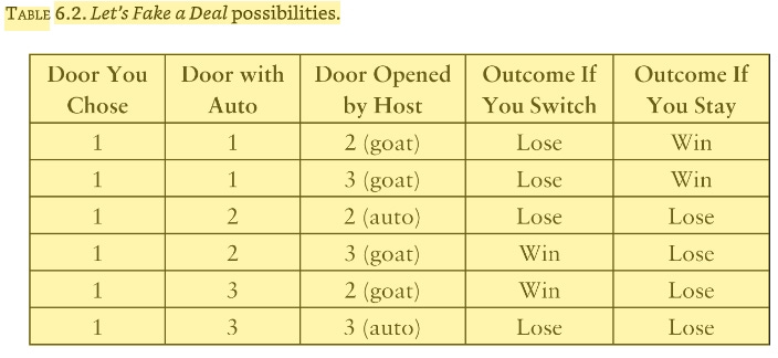
Now what happens if Monty Hall opens Door 3 and reveals a goat? This gives us some significant information: we must be in row 2 or 4 of the table. Focusing just on lines 2 and 4, we can see that the strategy of switching no longer offers us any advantage; we have a one-in-two probability of winning either way. So in the game Let’s Fake a Deal, all of Marilyn vos Savant’s critics would be right! Yet the data are the same in both games. The lesson is quite simple: the way that we obtain information is no less important than the information itself.

Ananthaswamy then describes how this “Monty Hall” puzzle brings to the fore two different ways of viewing probability:

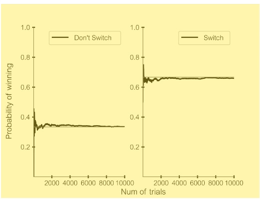
Encapsulated in this story about the Monty Hall dilemma is the tale of an eternal dispute between two ways of thinking about probability: frequentist and Bayesian. The former approach, which makes use of the simulation, is what seemingly convinced Erdős. The frequentist notion of the probability of occurrence of an event (say, a coin coming up heads) is simply to divide the number of times the event occurs by the total number of trials (the total number of coin flips). When the number of trials is small, the probability of the event can be wildly off from its true value, but as the number of trials becomes very large, we get the correct measure of the probability. The following figure shows the results of ten thousand trials of the Monty Hall dilemma. (Data scientist Paul van der Laken shows how to plot the probabilities of winning if you switch and if you don’t switch. This is one version.) You can see clearly that when the number of trials is small, the probabilities fluctuate. But they settle into the correct values as the trials go beyond about four thousand: 0.67, or two-thirds, for switching, and 0.33, or one-third, for not switching. But simulations are not the only way of answering such questions. Another approach is to rely on Bayes’s theorem, one of the cornerstones of probability theory and, indeed, of machine learning.

Ananthaswamy then describes the outlines of Bayes’s theorem:

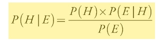
Bayes’s theorem gives us a way to draw conclusions, with mathematical rigor, amid uncertainty. It’s best to understand the theorem using a concrete example. Consider a test for some disease that occurs in only about 1 in 1,000 people. Let’s say that the test is 90 percent accurate, meaning that it comes back positive nine out of ten times when the person has the disease and that it is negative nine out of ten times when the person doesn’t have the disease. So, it gives false negatives 10 percent of the time and false positives 10 percent of the time. For the sake of simplicity, the rate of true positives (the sensitivity of the test) and the rate of true negatives (the specificity) are taken to be the same in this example; in reality, they can be different. Now you take the test, and it’s positive. What’s the chance you have the disease? We assume that the subject being tested—“ you” in this case— has been picked at random from the population. Most of us would say 90 percent, because the test is accurate 9 out of 10 times. We’d be wrong. To calculate the actual probability that one has the disease given a positive test, we need to take other factors into account. For this, we can use Bayes’s theorem. The theorem allows us to calculate the probability of a hypothesis H (you have the disease) being true, given evidence E (the test is positive). This is written as P( H | E): the probability of H given E. Bayes’s theorem says:

Let’s unpack the various terms on the right- hand side of the equation.

P( H): The probability that someone picked at random from the population has the disease. This is also called the prior probability (before taking any evidence into account). In our case, we can assume it is 1⁄1000, or 0.001, based on what’s been observed in the general population thus far.

P( E | H): The probability of the evidence given the hypothesis or, to put it simply, the probability of testing positive if you have the disease. We know this. It’s the sensitivity of the test: 0.9.

P( E): The probability of testing positive. This is the sum of the probabilities of two different ways someone can test positive given the background rate of the disease in the population. The first is the prior probability that one has the disease (0.001) multiplied by the probability that one tests positive (0.9), which equals 0.0009. The second is the prior probability that one doesn’t have the disease (0.999) times the probability that one tests positive (0.1), which equals 0.0999.

So, P( E) = 0.0009 + 0.0999 = 0.1008

So, P( H | E) = 0.001 × 0.9 / 0.1008 = 0.0089, or a 0.89 percent chance.

That’s way lower than the 90 percent chance we intuited earlier. This final number is called the posterior probability: It’s the prior probability updated given the evidence. To get a sense of how the posterior probability changes with alterations to the accuracy of the test, or with changes in the background rate of the disease in the population, let’s look at some numbers:

For a test accuracy rate of 99 percent— only 1 in 100 tests gives a false positive or false negative— and a background rate of disease in the population of 1 in 1,000, the probability that you have the disease given a positive test rises to 0.09. That’s almost a 1- in- 10 chance.

For a test accuracy rate of 99 percent (1 in 100 tests gives a false positive or false negative), and a background rate of disease in the population of 1 in 100 (the disease has become more common now), the probability that you have the disease given a positive test rises to 0.5. That’s a 50 percent chance.

Improve the test accuracy to 99.9 percent and keep the background rate at 1 in 100, and we get a posterior probability of 0.91. There’s a very high chance you have the disease if you tested positive.

With this whirlwind introduction to Bayes’s theorem, we are ready to tackle the Monty Hall problem. (This is a bit involved. Feel free to skip to the end of this section if you think it’s too much, though it’s quite revealing to see how Bayes’s theorem gets us to Marilyn vos Savant’s answer.)

We start by assuming that the car is hidden at random behind one of the three doors.

Let’s start by stating our hypothesis and our priors. We pick Door No. 1. The host opens Door No. 3, behind which is a goat. We must figure out whether it’s worth switching our guess from Door No. 1 to Door No. 2, to maximize our chances of choosing the door that hides the car. To do this, we must figure out the probabilities for two hypotheses and pick the higher of the two.

The first hypothesis is:

Car is behind Door No. 1, given that host has opened Door No. 3 and revealed a goat. The second hypothesis is: Car is behind Door No. 2, given that host has opened Door No. 3 and revealed a goat. Consider the probability of the first hypothesis:

P (H = car is behind Door No. 1 | E = host has opened Door No. 3, revealing a goat).

From Bayes’s theorem:

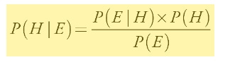
Where:

P (E | H): the probability that the host opens Door No. 3, given that the car is behind Door No. 1. At the start of the game, you picked Door No. 1. If the car is behind it, the host can see that and, hence, has a choice of two doors to open, either No. 2 or No. 3, both of which hide goats. The probability they’ll open one of them is simply 1/ 2.

P (H): the prior probability that the car is behind Door No. 1, before any door is opened. It’s 1/ 3.

P (E): the probability that the host opens Door No. 3. This must be carefully evaluated, given that the host knows that you have picked Door No. 1 and they can see what’s behind each door. So,

P (host picks Door No. 3) = P1 + P2 + P3

P1 = P (car is behind Door No. 1) × P (host picks Door No. 3, given car is behind Door No. 1) = P (C1) × P (H3 | C1)

P2 = P (car is behind Door No. 2) × P (host picks Door No. 3, given car is behind Door No. 2) = P (C2) × P( H3 | C2)

P3 = P (car is behind Door No. 3) × P (host picks Door No. 3, given car is behind Door No. 3) = P (C3) × P( H3 | C3)

Take each part of the right-hand side of the equation:

P1: P (C1) × P (H3 | C1).

P (C1) = P (car is behind Door No. 1) = 1/ 3.

P (H3 | C1)— if the car is behind Door No. 1, then the probability that the host opens Door No. 3 is 1/ 2. They could have picked either Door No. 2 or Door No. 3.

So, P1 = 1/ 3 × 1/ 2 = 1/ 6.

P2: P (C2) x P (H3 | C2). P (C2) = P (car is behind Door No. 2) = 1/ 3.

P (H3 | C2)— if the car is behind Door No. 2, then the probability that the host opens Door No. 3 is 1, because they cannot pick Door No. 2, otherwise it’ll reveal the car.

So, P2 = 1/ 3 × 1 = 1/ 3

P3: P (C3) × P (H3 | C3).

P (C3) = P (car is behind Door No. 3) = 1/ 3.

P (H3 | C3)— if the car is behind Door No. 3, then the probability that the host opens Door No. 3 is 0, otherwise it’ll reveal the car.

So, P3 = 1/ 3 × 0 = 0

So, P (E) = P1 + P2 + P3 = 1/ 6 + 1/ 3 + 0 = 3/ 6 = 1/ 2

We can now calculate the probability that hypothesis 1 is true, given the evidence:

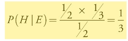
The probability that the car is behind the door you have picked is 1/ 3.

Now let’s calculate the probability for the second hypothesis: The car is behind Door No. 2 given that the host has opened Door No. 3, revealing a goat. We can do a similar analysis.

P (E | H): Probability that the host opens Door No. 3, given that the car is behind Door No. 2. The host cannot open Door No. 2. They have to open Door No. 3, so the probability of this event is 1.

P (H): The prior probability that the car is behind Door No. 2, before any door is opened. It’s 1/ 3.

P (E): As computed before, it’s ½.

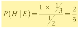
Very clearly, the second hypothesis— that the car is behind Door No. 2, given that the host has opened Door No. 3— has a higher probability compared to the probability that the car is behind Door No. 1 (your original choice). You should switch doors!  If all this feels counterintuitive and you still refuse to change your choice of doors, it’s understandable. Probabilities aren’t necessarily intuitive. But when machines incorporate such reasoning into the decisions they make, our intuition doesn’t get in the way.

In the next essay in this series, we’ll get to know more about Thomas Bayes himself, and some of the other practical applications of Bayes’s theorem, before returning to more of the math and mechanics of machine learning.