Machine Learning, ChatGPT, and Bayes’s Theorem – Part 4

How figuring out whether James Madison wrote certain essays led to ChatGPT.

This continues an essay series on how the sort of AI that entails what’s become called “machine learning” works, using Anil Ananthaswamy’s book Why Machines Learn: The Elegant Math Behind Modern AI to help explain things.  This essay explores how figuring out whether James Madison wrote certain essays led to ChatGPT.

As Ananthaswamy writes:

One of the first large-scale demonstrations of using Bayesian reasoning for machine learning was due to two statisticians, Frederick Mosteller and David Wallace, who used the technique to figure out something that had been bothering historians for centuries: the authorship of the disputed Federalist Papers. Months after the U.S. Constitution was drafted in Philadelphia in the summer of 1787, a series of essays, published anonymously under the pen name “Publius,” began appearing in newspapers in New York State. Seventy-seven such essays were published, written to convince New Yorkers to ratify the Constitution. These essays, plus eight more, for a total of eighty-five, were then published in a two-volume set titled The Federalist: A Collection of Essays, Written in Favour of the New Constitution, as Agreed upon by the Federal Convention, September 17, 1787. Eventually, it became known that the essays had been written by Alexander Hamilton, John Jay, and James Madison, three of the “founding fathers” of the United States. About two decades later, and after Hamilton had died (following a fatal duel between him and Aaron Burr, the then-U.S. vice president), the essays began to be assigned to individual authors. For seventy of the papers, the writers were known. But of the remaining papers, twelve were thought to have been written by either Hamilton or Madison, and three were thought to have been co-authored. You’d think that Madison, who was still alive, would have clearly identified the authors of each paper. But as Frederick Mosteller writes in The Pleasures of Statistics, “the primary reason the dispute existed is that Madison and Hamilton did not hurry to enter their claims. Within a few years after writing the essays, they had become bitter political enemies and each occasionally took positions opposing some of his own Federalist writings.” They behaved like lawyers writing briefs for clients, Mosteller writes: “They did not need to believe or endorse every argument they put forward favoring the new Constitution.” Consequently, the authorship of these fifteen documents remained unresolved. In 1941, Mosteller and a political scientist named Frederick Williams decided to tackle the problem. They looked at the lengths of sentences used by Madison and Hamilton in the papers whose authorship was not in dispute. The idea was to identify each author’s unique “signatures”—maybe one author used longer sentences than the other—and then use those signatures to check the sentence lengths of the disputed papers and, hence, their authorship. But the effort led nowhere. “When we assembled the results for the known papers the average lengths for Hamilton and Madison were 34.55 and 34.59, respectively—a complete disaster because these averages are practically identical and so could not distinguish authors.” Mosteller and Williams also calculated the standard deviation (SD), which provided a measure of the spread of the sentence lengths. Again, the numbers were very close. The SD for Hamilton was 19, and 20 for Madison. If you were to draw the normal distribution of sentence lengths for each author, the two curves would overlap substantially, providing little discriminatory power. This work became a teaching moment. Mosteller, while lecturing at Harvard, used this analysis of The Federalist Papers to educate his students on the difficulties of applying statistical methods. By the mid-1950s, Mosteller and statistician David Wallace, who was at the University of Chicago, began wondering about using Bayesian methods for making inferences. At the time, there were no examples of applying Bayesian analysis to large, practical problems. It was about then that Mosteller received a letter from the historian Douglass Adair, who had become aware of the courses being taught by Mosteller at Harvard. Adair wanted Mosteller to revisit the issue of the authorship of The Federalist Papers. “[Adair]…was stimulated to write suggesting that I (or more generally, statisticians) should get back to this problem. He pointed out that words might be the key, because he had noticed that Hamilton nearly always used the form ‘while’ and Madison the form ‘whilst.’ The only trouble was that many papers contained neither of them,” Mosteller writes. “We were spurred to action.” One of their ideas that bore fruit was to look at so-called function words, words that have a function rather than a meaning—prepositions, conjunctions, and articles. First, they had to count the occurrence of such words in documents written by Hamilton and Madison. It was a laborious process. And so it went, a few thousand words at a time, until they had the counts for certain function words that appeared in a large number of articles written by Hamilton and Madison … Now it was time to figure out the authorship of one of the disputed papers. They used Bayesian analysis to calculate the probability of two hypotheses: (1) the author is Madison, and (2) the author is Hamilton. If hypothesis 1 has a greater probability, the author is more likely to be Madison. Otherwise, it’s Hamilton. Take one function word, say, “upon,” and calculate the probability of hypothesis 1 given the word and hypothesis 2 given the word, and ascribe authorship appropriately. Of course, using multiple words at once makes the analysis sharper. The key insight here is that given a bunch of known documents by Madison, the usage of some word, such as “upon,” follows a distribution. Madison used the word more in some documents, less so in others. The same can be said of Hamilton. As we saw in the issue with sentence length, if these distributions are alike, they cannot be used to tell the authors apart. But if they are different, they possess the power to discriminate. Mosteller makes this point eloquently: “The more widely the distributions of rates [of words] of the two authors are separated, the stronger the discriminating power of the word. Here, [the word] by discriminates better than [the word] to, which in turn is better than [the word] from.” The results were unanimous. “By whatever methods are used, the results are the same: overwhelming evidence for Madison’s authorship of the disputed papers. Our data independently supplement the evidence of the historians. Madison is extremely likely, in the sense of degree of belief, to have written the disputed Federalist papers, with the possible exception of paper number 55, and there our evidence yields odds of 80 to 1 for Madison—strong, but not overwhelming.”

The development of the process to determine Federalist Paper authorship jumpstarted the quest for an AI word predictor.  As Ananthaswamy writes:

Patrick Juola, professor of computer science at Duquesne University in Pittsburgh, Pennsylvania, and a modern-day expert in stylometry (the use of the statistics of variations in writing style to determine authorship), said that Mosteller and Wallace’s work was a seminal moment for statisticians. “It was very influential in statistical theory. And they were justifiably lauded,” Juola told me. “Historians had been looking at the problem for a hundred years. And the historians had mostly come to the same decisions that Mosteller and Wallace did. And what made [their] study so groundbreaking was [that] for the first time, this was done in a completely objective, algorithmic fashion, which is to say it was machine learning.”

Machine learning has gotten so good at discerning and predicting patterns that its utility in creating computer code is already being reflected in the coding job market. As Brent Orrell writes:

The most recent figures from the Federal Reserve Bank of New York are startling: Unemployment among people with computer engineering and computer science degrees is at least twice as high as that of graduates in fields like psychology, philosophy, art history and early childhood education.

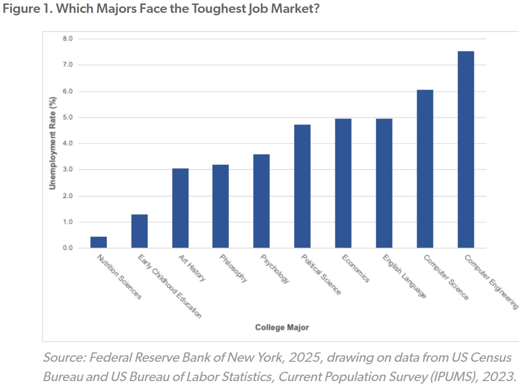
As with all economic figures, there are nuances. Although the unemployment rate for computer scientists and engineers is high, their underemployment rate (i.e., the share not working in roles that fully utilize their skills) is significantly lower than that of liberal arts majors. For example, the underemployment rate for computer engineering graduates is only 16.5 percent, compared to 46.8 percent for nutrition sciences graduates. This suggests that, while nontechnical majors may be more likely to be employed, they may also be more likely to be taking jobs that are unrelated to the degrees they received.

A forerunner to ChatGPT’s algorithms is something called the “nearest neighbor rule”:

ML [machine learning] algorithms don’t get much simpler than the nearest neighbor rule for classifying data. Especially considering the algorithm’s powerful abilities. Let’s start with a mock dataset of gray circles and black triangles:

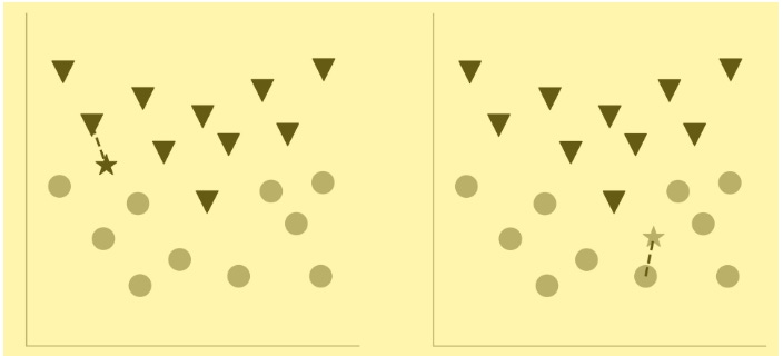
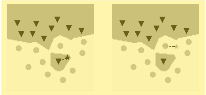
Recall the perceptron algorithm. It will fail to tell apart the circles from the triangles, because this dataset is not linearly separable: There’s no single straight line you can draw to delineate the two classes of data. A naïve Bayes classifier can find a windy line that separates the circles from the triangles, though. We’ll come back to that in a bit, but for now, let’s tackle the nearest neighbor algorithm. The problem we must solve is this: When given a new data point, we have to classify it as either a circle or a triangle … The nearest neighbor algorithm, in its simplest form, essentially plots that new data point and calculates its distance to each data point in the initial dataset, which can be thought of as the training data. (We’ll use the Euclidean distance measure for our purposes.) If the data point nearest to the new data is a black triangle, the new data is classified as a black triangle; if it’s a gray circle, the new data is classified as a gray circle. It’s as simple as that. The following two panels show how a new data point is labeled based on its nearest neighbor. (The new data point is shown as a star, but is colored either gray or black, depending on whether it’s classified as a gray circle or a black triangle.) The original dataset is the same as the one shown in the previous panel.

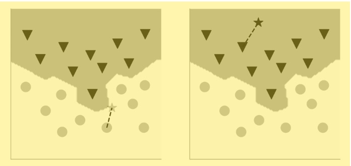
Going back to the perceptron algorithm, recall that the linearly separating hyperplane divides the coordinate space into two regions. The nearest neighbor algorithm does the same, except in this case, the boundary between the two regions is not a straight line (or a hyperplane in higher dimensions). Rather, it’s squiggly, nonlinear. Look at the two plots above, and you can imagine a boundary such that if the new data point fell on one side of the boundary, it’d be closer to a gray circle, or else to a black triangle. Here’s what the boundary looks like for the same dataset when the NN algorithm examines just one nearest neighbor. You can see that a new data point (a gray star) that’s closest to a gray circle lies in the region that contains all the gray circles, and one that’s closest to a black triangle lies in the region containing all the black triangles.

This simple algorithm—we’ll come to the details in a moment—achieves something quite remarkable: It finds a nonlinear boundary to separate one class of data from another. But the simplicity of the algorithm that uses just one nearest neighbor belies a serious problem. Can you figure it out before reading further …

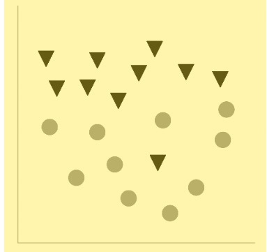
To help understand the potential problem, consider another dataset (shown above), one that includes a data point that’s misclassified by humans as a black triangle and that lies amid the gray circles. What do you think might happen, in terms of finding the boundary separating the circles from the triangles? The machine, it must be said, would have no way of knowing that the errant black triangle had been misclassified as such. Given the data, the algorithm will find a nonlinear boundary that’s quite intricate. Here’s the solution:

Notice how the nonlinear boundaries split up the coordinate space into more than two gray-and-white regions. There’s a small “island” surrounding the misclassified black triangle. If your new data point is within that small island, it’ll get classified as a black triangle even though it’s surrounded by gray circles. What we have seen is an example of what ML researchers call overfitting. Our algorithm has overfit the data. It finds a boundary that doesn’t ignore even a single erroneous outlier. This happens because the algorithm is paying attention to just one nearest neighbor. There’s a simple fix, however, that addresses this problem. We can simply increase the number of nearest neighbors against which to compare the new data point. The number of neighbors must be odd (say, three or five or more). Why an odd number? Well, because if it were even, we could end up with a tie, and that’s of no use. An odd number ensures we’ll get an answer, right or wrong. This is assuming that we are working only with data that can be clustered into two classes (in this case, the gray circles and the black triangles). Here’s the same dataset, but now the algorithm looks for three nearest neighbors and classifies the new data point based on the majority vote:

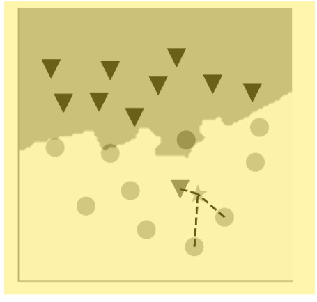
The nonlinear boundary no longer gives undue attention to the one lone triangle amid the circles. If a new data point were to fall near this lone triangle, it’d still be classified as a circle, because the triangle would be outvoted by the nearby circles. The boundary has become somewhat smoother; it’s not contorting to account for the noise in the data, which in our case is the misclassified triangle. Such smoother boundaries, using a larger number of nearest neighbors, are more likely to correctly classify a new data point when compared with the boundary we got using just one nearest neighbor.

And this is relevant to our daily lives today:

What can such a simple algorithm achieve? How about all the stuff that you get asked to buy on the internet? If companies, which shall not be named, want to recommend that you buy certain books or watch certain movies, they can do this by representing you as a vector in some high-dimensional space (in terms of your taste in books or movies), find your nearest neighbors, see what they like, and recommend those books or movies to you.

As Ananthaswamy explains, successive machine learning processes have gotten so sophisticated that, while researchers see that they largely work, they often don’t understand quite how they work, or the mathematics that might govern their operations:

The ignorance [researchers] and others admit to is mostly about not knowing the mathematical underpinnings of the observed behavior of neural networks in this new, over-parameterized regime. This is somewhat unexpected from ML research. In fact, much of this book has celebrated the fact that traditional machine learning has had a base of well-understood mathematical principles, but deep neural networks—especially the massive networks we see today—have upset this applecart. Suddenly, empirical observations of these networks are leading the way. A new way of doing AI seems to be upon us … One of the most elegant demonstrations of empirical observations in need of theory is grokking … [That is] the story of the OpenAI researcher who came back from a vacation and found that the neural network, which had continued training, had learned something deep about adding two numbers, using modulo-97 arithmetic. “It was not something we were expecting to find at all,” Alethea Power told me. “Initially, we thought it was a fluke and dug deeper into it. It turned out to be something that happens pretty reliably.” The neural network that Power and colleagues were using was called a transformer, a type of architecture that’s especially suited to processing sequential data. LLMs such as ChatGPT are transformers; GPT stands for “generative pre-trained transformer.” Given a sequence of, say, ten words and asked to predict the next most plausible word, a transformer has the ability to “pay attention” to all the words at once and also to the order of the words and not just treat them as some arbitrary jumble. Of course, commercial LLMs are behemoths, with tens or even hundreds of billions of parameters. In contrast, the transformer that Power’s team was using was tiny, with fewer than half a million parameters.

Although AI neural networks are getting much better at their jobs, there’s no reason to fear their ever gaining consciousness as humans understand it.  As Ananthaswamy writes:

There’s considerable debate over whether neural networks alone (possibly with new architectures no one has dreamed of yet and training methods that are ever more effective) will get us from ML-based pattern recognition to true AI that can reason effectively. But here’s something that puts these issues into perspective. In June 2022, Google announced a large language called Minerva. It was built on top of Google’s own LLM, called the Pathways Language Model (PaLM), a 540-billion-parameter model—at the time, the largest densely connected model. PaLM was trained on about 780 billion “tokens” of data taken from the internet. (Think of a token as a word or a digit.) Google researchers then fine-tuned PaLM by training it further on 118 gigabytes of data, mainly “scientific papers from the arXiv preprint server and web pages that contain mathematical expressions.” Both PaLM and Minerva were trained using self-supervised learning, meaning they were taught to predict masked tokens in some sequence of tokens that appeared in the training data. They were not taught to explicitly reason or solve math problems. Even so, here’s what happened when Minerva was posed this question (taken from something called the “MATH” dataset of about 12,500 high school–level mathematics questions):

Question: A line parallel to y = 4x + 6 passes through (5, 10). What is the y-coordinate of the point where this line crosses the y-axis?

Minerva: The line is parallel to y = 4x + 6, which means that it has the same slope as y = 4x + 6. Since the line passes through (5, 10), we can use the point-slope form of a line to find the equation of the line:

y - 10 = 4(x - 5)

y - 10 = 4x – 20

y = 4x – 10

Now that we have the equation of the line, we can find the y-coordinate of the point where the line crosses the y-axis by substituting x = 0 into the equation: y = 4 × 0 - 10 = -10.

Minerva was the first LLM to correctly answer about 50 percent of the questions in the MATH dataset; of course, it got the other questions wrong. But think about what Minerva is doing. It takes the question, turns it into a sequence of tokens, and then simply predicts what follows, token by token. Out comes what appears to be a reasoned answer.

While AI machine learning is constantly improving, its physical mechanisms in no way resemble how human brains work.  As Ananthaswamy explains:

An LLM is trained to predict the next word, given a sequence of words. (In practice, the algorithm chunks the input text into tokens, which are contiguous characters of some length that may or may not be entire words. We can stick with words with no loss of generality.) These sequences of words—say, a fragment of a sentence or an entire sentence or even a paragraph or paragraphs—are taken from a corpus of training text, often scraped from the internet. Each word is first converted into a vector that’s embedded in some high-dimensional space, such that similar words—for some notion of similarity—are near each other in that space. There are pre-trained neural networks that can do this; it’s a process called word embedding. For every sequence of words presented to an LLM as vectors, the LLM needs to learn to predict the next word in the sequence. Here’s one way to train an LLM, which is a monstrously large deep neural network with tens or hundreds of billions of parameters. We know that the neural network is a function approximator. But what is the function we want to approximate? Turns out it’s a conditional probability distribution. So, given a sequence of (n-1) input words, the neural network must learn to approximate the conditional probability distribution for the nth word, P(wn| w1, w2,…, wn-1), where the nth word can be any word in the vocabulary, V. For example, if you gave the LLM the sentence “The dog ate my ______,” the LLM must learn the values for P (cat | The, dog, ate, my), P (biscuit | The, dog, ate, my), P (homework | The, dog, ate, my), and so on. Given the occurrences of this phrase in the training data, the probability distribution might peak for the word “homework,” have much smaller peaks for other likely words, and be near zero for the unlikely words in the vocabulary. The neural network first outputs a set of V numbers, one number for each possible word to follow the input sequence. (I’m using V to denote the vocabulary and V its size.) This V-dimensional vector is then passed through something called a softmax function (almost but not quite like the sigmoid we saw earlier), which turns each element of the vector into a probability between 0 and 1 and ensures that the total probability adds up to 1. This final V-dimensional vector represents the conditional probability distribution, given the input; it gives us the probability for each word in the vocabulary, if it’s to follow the sequence of input words. There are many ways of sampling from this distribution, but let’s say we greedily sample to get the most likely next word. This next word is the neural network’s prediction. Once trained, the LLM is ready for inference. Now given some sequence of, say, 100 words, it predicts the most likely 101st word. (Note that the LLM doesn’t know or care about the meaning of those 100 words: To the LLM, they are just a sequence of text.) The predicted word is appended to the input, forming 101 input words, and the LLM then predicts the 102nd word. And so it goes, until the LLM outputs an end-of-text token, stopping the inference. That’s it! … An LLM is an example of generative AI. It has learned an extremely complex, ultra-high-dimensional probability distribution over words, and it is capable of sampling from this distribution, conditioned on the input sequence of words. There are other types of generative AI, but the basic idea behind them is the same: They learn the probability distribution over data and then sample from the distribution, either randomly or conditioned on some input, and produce an output that looks like the training data … [D]espite the cherry-picked examples I’ve shown, in which the LLMs produced the correct outputs, they do often spit out wrong answers, sometimes obviously wrong, at times with subtle mistakes that might be hard to catch if you aren’t an expert yourself. LLMs have serious applications. For example, LLMs fine-tuned on web pages containing programming code, are excellent assistants for programmers: Describe a problem in natural language, and the LLM will produce the code to solve it. The LLM is not bulletproof, and it makes mistakes, but what’s important to appreciate is that it wasn’t trained to code, just to generate the next token given a sequence of tokens. Yet, it can generate code. The gains in productivity for programmers cannot be denied … As exciting as these advances are, we should take all these correspondences between deep neural networks and biological brains with a huge dose of salt. These are early days. The convergences in structure and performance between deep nets and brains do not necessarily mean the two work in the same way; there are ways in which they demonstrably do not … [T]here are massive differences between biological brains and deep neural networks when it comes to energy efficiency. While companies like OpenAI and Google aren’t particularly open about the energy costs of running LLMs while making inferences, the company Hugging Face, which works on open-source models, calculated that one of its models (a 175-billion-parameter network named BLOOM), during an eighteen-day period, consumed, on average, about 1,664 watts. Compare that to the 20 to 50 watts our brains use, despite our having about 86 billion neurons and about 100 trillion connections, or parameters. On the face of it, it’s no comparison, really. (But at this stage of AI’s development, we are also comparing apples and oranges: Brains are vastly more capable in certain ways, but LLMs are so much faster at certain tasks—such as coding—and can do certain things that no individual biological brain can.)

Also, as Chivers describes, our bodies’ communication system does rely on a basic version of Bayesian reasoning:

[Y]ou can’t be a Bayesian without priors. Without some sense of how probable something was before you saw the evidence, you can’t make any claims about how likely it is after seeing the evidence … [Y]our senses predict the world, and when the world is as they predicted it, they don’t send any more signals. But when the predictions are wrong, they send signals higher up. This is crucial. At every level in the hierarchy, what we experience is what we predict. Those predictions are checked against reality. If reality agrees, fine. If it doesn’t, we have a prediction error, and then signals are sent further up.

In the next essay in this series, we’ll use Tom Chivers’ book Everything Is Predictable: How Bayesian Statistics Explain Our World to help summarize what we’ve explored so far, and to describe some of AI machine learning’s practical applications today.