Machine Learning, ChatGPT, and Bayes’s Theorem – Part 1

An introduction to machine learning.

In previous essay series, we explored various dysfunctions in way medical and other scientific research is conducted.  Some have pointed to artificial (computer) intelligence (“AI”) as a means of surmounting some of the barriers to progress caused by some unfortunate human tendencies, such as those toward bureaucracy and tribalism.

On the one hand, some have touted AI as:

going to have some if its biggest effects on biology. Biological pathways are among the most complex in all of science. People are good at handling two or maybe three variable problems but just keeping three variables and their interactions in one’s head is difficult. AIs with access to vast databases of genes, proteins, networks and so forth will enable new simulations and learning as has already happened with protein folding [a way of making proteins capable of functioning in a biological process].

And Michael Bhaskar, in his book Human Frontiers: The Future of Big Ideas in an Age of Small Thinking, writes:

The significance [of AI] is twofold. First it suggests a way out of the burden of knowledge problem. This is a system specifically designed to cut through a mass of learning impossible for any human to digest. As knowledge accumulates, so technology like Word2vec can sift through it. Second, it shows how even at a comparatively early stage, AI has enormous potential to make significant, useful discoveries improbable with the old toolset.

On the other hand, such predictions often fail to live up to their hype.  As reported by the Globe and Mail:

Deep Genomics is the latest drug company to announce that AI hasn’t helped them to develop drugs despite testing more than 200 million molecules proposed by AI. Today, it “has zero drugs in clinical trials and many of its plans have blown up. The company halted its Wilson disease program, ditched dozens of its machine learning models, appointed a new chief executive and is pursuing a different approach to using AI. It’s also open to a sale.” “AI was supposed to revolutionize drug discovery. It hasn’t. Not yet, anyway. Machine learning promised to speed up a lengthy and fraught process, and achieve breakthroughs beyond the capabilities of the human mind. But there are no drugs solely designed by AI in the market today, and companies that have used AI to assist with development have suffered setbacks.” Deep Genomics founder Brendan Frey says: “AI has really let us all down in the last decade when it comes to drug discovery. We’ve just seen failure after failure.” “The blunt assessment is shocking coming from Mr. Frey” because “he has been studying machine learning since the 1990s, and he is the co-author of more than 200 papers and a co-founder of the Vector Institute, a nerve centre for AI research in Canada.” … Recursion Pharmaceuticals in the United States said that it would find 100 clinical candidates in its first 10 years. A decade later, it has five in trials. In August, Recursion and Exscientia announced a merger, after years of cratering share prices … The setbacks in drug development could hold lessons for other industries hoping that AI will unlock massive productivity gains. Molecular biology is immensely more complicated than building a chatbot, of course, but new technology is anything but straightforward.

But as more and more people use tools like ChatGPT to answer various questions, with increasingly accurate and helpful results, it’s worth exploring exactly how the sort of AI that constitutes what’s become called “machine learning” works.  That’s the subject of this series of essays, in which we’ll largely use Anil Ananthaswamy’s book Why Machines Learn: The Elegant Math Behind Modern AI, and Tom Chivers’ book Everything Is Predictable: How Bayesian Statistics Explain Our World, to help explain things.

As Ananthaswamy writes:

[E]legant mathematics and algorithms … have, for decades, energized and excited researchers in “machine learning,” a type of AI that involves building machines that can learn to discern patterns in data without being explicitly programmed to do so. Trained machines can then detect similar patterns in new, previously unseen data, making possible applications that range from recognizing pictures of cats and dogs to creating, potentially, autonomous cars and other technology. Machines can learn because of the extraordinary confluence of math and computer science, with more than a dash of physics and neuroscience added to the mix … [AI involves] equations and concepts from at least four major fields of mathematics—linear algebra, calculus, probability and statistics, and optimization theory—to acquire the minimum theoretical and conceptual knowledge necessary to appreciate the awesome power we are bestowing on machines. It is only when we understand the inevitability of learning machines that we will be prepared to tackle a future in which AI is ubiquitous, for good and for bad … But what do these terms mean? What are “patterns” in data? What does “learning about these patterns” imply? Let’s start by examining this table: Each row in the table is a triplet of values for variables x1, x2, and y. There’s a simple pattern hidden in this data: In each row, the value of y is related to the corresponding values of x1 and x2. See if you can spot it before reading further.

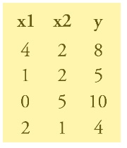
In this case, with a pencil, paper, and a little effort one can figure out that y equals x1 plus two times x2.

y = x1 + 2x2

A small point about notation: We are going to dispense with the multiplication sign (“×”) between two variables or between a constant and a variable. For example, we’ll write 2 × x2 as 2x2 and x1 × x2 as x1x2.

Finding patterns is nowhere near as simple as this example is suggesting, but it gets us going. In this case, the correlation, or pattern, was so simple that we needed only a small amount of labeled data. But modern ML [machine learning] requires orders of magnitude more—and the availability of such data has been one of the factors fueling the AI revolution.

Back in the 1950’s, Frank Rosenblatt developed a machine called the Perceptron.  As Ananthaswamy explains:

Rosenblatt eventually built the Mark I Perceptron. The device had a camera that produced a 20x20-pixel image. The Mark I, when shown these images, could recognize letters of the alphabet. But saying that the Mark I “recognized” characters is missing the point, Nagy said. After all, optical character recognition systems, which had the same abilities, were commercially available by the mid-1950s. “The point is that Mark I learned to recognize letters by being zapped when it made a mistake!” [George] Nagy would say in his talks. But what exactly is a perceptron, and how does it learn? … To understand how this works, consider a perceptron that seeks to classify someone as obese, y = +1, or not-obese, y = -1. The inputs are a person’s body weight, x1, and height, x2. Let’s say that the dataset contains a hundred entries, with each entry comprising a person’s body weight and height and a label saying whether a doctor thinks the person is obese according to guidelines set by the National Heart, Lung, and Blood Institute. A perceptron’s task is to learn the values for w1 and w2 and the value of the bias term b, such that it correctly classifies each person in the dataset as “obese” or “not-obese.” Note: We are analyzing a person’s body weight and height while also talking about the perceptron’s weights (w1 and w2); keep in mind these two different meanings of the word “weight” while reading further. Once the perceptron has learned the correct values for w1 and w2 and the bias term, it’s ready to make predictions. Given another person’s body weight and height—this person was not in the original dataset, so it’s not a simple matter of consulting a table of entries—the perceptron can classify the person as obese or not-obese. Of course, a few assumptions underlie this model, many of them to do with probability distributions, which we’ll come to in subsequent chapters. But the perceptron makes one basic assumption: It assumes that there exists a clear, linear divide between the categories of people classified as obese and those classified as not-obese. In the context of this simple example, if you were to plot the body weights and heights of people on an xy graph, with weights on the x-axis and heights on the y-axis, such that each person was a point on the graph, then the “clear divide” assumption states that there would exist a straight line separating the points representing the obese from the points representing the not-obese. If so, the dataset is said to be linearly separable. Here’s a graphical look at what happens as the perceptron learns.

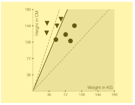
We start with two sets of data points, one characterized by black circles (y = +1, obese) and another by black triangles (y = -1, not-obese). Each data point is characterized by a pair of values (x1, x2), where x1 is the body weight of the person in kilograms, plotted along the x-axis, and x2 is the height in centimeters, plotted along the y-axis. The perceptron starts with its weights, w1 and w2, and the bias initialized to zero. The weights and bias represent a line in the xy plane. The perceptron then tries to find a separating line, defined by some set of values for its weights and bias, that attempts to classify the points. In the beginning, it classifies some points correctly and others incorrectly. Two of the incorrect attempts are shown as the gray dashed lines. In this case, you can see that in one attempt, all the points lie to one side of the dashed line, so the triangles are classified correctly, but the circles are not; and in another attempt, it gets the circles correct but some of the triangles wrong. The perceptron learns from its mistakes and adjusts its weights and bias. After numerous passes through the data, the perceptron eventually discovers at least one set of correct values of its weights and its bias term. It finds a line that delineates the clusters: The circles and the triangles lie on opposite sides. This is shown as a solid black line separating the coordinate space into two regions (one of which is shaded gray). The weights learned by the perceptron dictate the slope of the line; the bias determines the distance, or offset, of the line from the origin. Once the perceptron has learned the correlation between the physical characteristics of a person (body weight and height) and whether that person is obese (y = +1 or -1), you can give it the body weight and height of a person whose data weren’t used during training, and the perceptron can tell you whether that person should be classified as obese. Of course, now the perceptron is making its best prediction, having learned its weights and bias, but the prediction can be wrong. Can you figure out why? See if you can spot the problem just by looking at the graph. (Hint: How many different lines can you draw that succeed in separating the circles from the triangles?) As we’ll see, much of machine learning comes down to minimizing prediction error … What’s described above is a single perceptron unit, or one artificial neuron. It seems simple, and you may wonder what all the fuss is about. Well, imagine if the number of inputs to the perceptron went beyond two: (x1, x2, x3, x4, and so on), with each input (xi) getting its own axis. You can no longer do simple mental arithmetic and solve the problem. A line is no longer sufficient to separate the two clusters, which now exist in much higher dimensions than just two. For example, when you have three points (x1, x2, x3), the data is three-dimensional: you need a 2D plane to separate the data points. In dimensions of four or more, you need a hyperplane (which we cannot visualize with our 3D minds). In general, this higher-dimensional equivalent of a 1D straight line or a 2D plane is called a hyperplane.

Ananthaswamy continues the historical narrative:

But then, [Marvin] Minsky and [Seymour] Papert’s 1969 book, which provided such a firm mathematical foundation for research on perceptrons, also poured an enormous amount of cold water on it. Among the many proofs in their book, one addresses a very simple problem that a single layer of perceptrons could never solve: the XOR problem. Look at the four data points shown in the figure below.

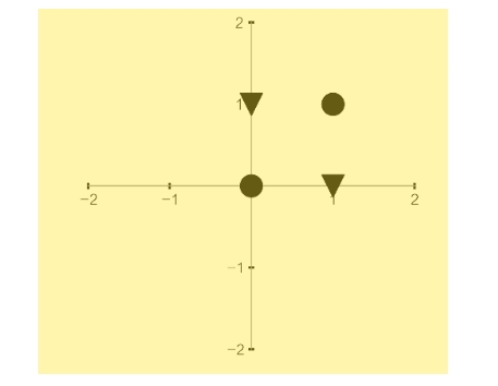
No straight line you can draw will separate the circles from the triangles. The points (x1, x2) in this case are: (0, 0), (1, 0), (1, 1) and (0, 1). For the perceptron to separate the circles, represented by the points (0, 0) and (1, 1), from the triangles, represented by (1, 0) and (0, 1), it must be able to generate an output y = 1 when both x1 and x2 are 0 or both x1 and x2 are 1, and an output y = -1 otherwise. No such straight line exists, something that is easy to see visually. Minsky and Papert proved that a single layer of perceptrons cannot solve such problems … [But now] [i]t’s possible to solve the XOR problem if you stack perceptrons, such that the output of one feeds into the input of another. These would be so-called multi-layer perceptrons.

Anansaswamy then describes how another big advance for machine learning came when, in 1959:

Bernard Widrow, a young academic on the cusp of turning thirty, was in his office at Stanford University when a graduate student named Marcian “Ted” Hoff came looking for him. The young man arrived highly recommended. The day before, a senior professor at Stanford had reached out to Widrow on Hoff’s behalf, saying, “I’ve got this student named Ted Hoff. I can’t seem to get him interested [in my research]; maybe he’d be interested in what you’re doing. Would you be willing to talk with him?” Widrow replied, “Sure, happy to.”“So, the next day, knocking on my door was Ted Hoff,” Widrow told me. Widrow welcomed him in and proceeded to discuss his work, which was focused on adaptive filters—electronic devices that learn to separate signals from noise—and the use of calculus to optimize such filters. As Widrow chalked up the math on the blackboard, Hoff joined in, and soon the conversation morphed into something more dramatic. During that discussion, the two invented what came to be called the least mean squares (LMS) algorithm, which has turned out to be one of the most influential algorithms in machine learning, having proven foundational for those figuring out how to train artificial neural networks … Widrow … turned to something more concrete: adaptive filters that could learn to remove noise from signals. He was particularly interested in the digital form of adaptive analog filters developed by Norbert Wiener. To understand Wiener’s analog filter, consider some continuously varying (hence analog) signal source. Some noise is added to the signal, and the filter’s job is to tell signal from noise. Wiener’s filter theory showed how this could be done. Others adapted the theory to digital signals. Instead of being continuous, digital signals are discrete, meaning they have values only at certain points in time (say, once every millisecond). Widrow wanted to build a digital filter, but one that could learn and improve over time. In other words, it would learn from its mistakes and become a better version of itself. At the heart of such an adaptive filter is a nifty bit of calculus. Imagine that the filter, at any given time, makes an error. Let’s assume that we are able to keep track of such errors for ten time steps. We must reduce the error the filter makes by looking at its previous ten errors and adjusting its parameters. One measure of the mistakes is simply the average of the previous ten errors. However, errors can be positive or negative, and if you just add them to take the average, they can cancel each other out, giving the wrong impression that the filter’s working well. To avoid this, take the square of each error (thus turning it into a positive quantity) and then take the average of the squares of the errors. The goal is to minimize this “mean squared error” (MSE) with respect to the parameters of the filter. To restate, we must change the values of the filter’s parameters at each time step such that the average, or mean, of the squared errors of the past, say, ten steps is minimized. Understanding how this works requires delving into some simple calculus and learning a method that was first proposed in 1847 by Baron Augustin-Louis Cauchy, a French mathematician, engineer, and physicist. It’s called the method of steepest descent.

Ananthswamy then describes how the method of steepest descent works:

If you have seen pictures of—or, better yet, visited—rice paddies on hillsides, particularly in China, Japan, and Vietnam, you may have marveled at the flat terraces cut into the sides of the hills. If we walk along any one terrace, we remain at the same elevation. The edges of the terraces trace the contours of the terrain. Imagine standing on some terrace way up a hillside.

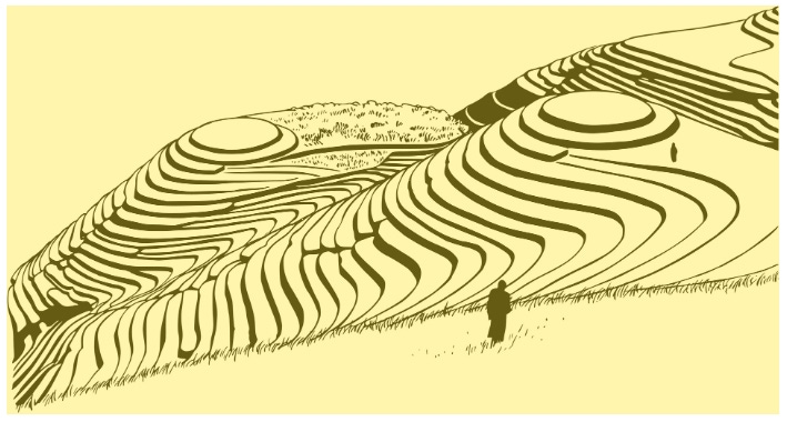
Down in the valley below is a village. We have to get to the village, but it’s getting dark, and we can see only a few feet ahead of us. Let’s say the hillside is not too steep and that it’s possible to clamber down even the steepest parts. How will we proceed? We can stand at the edge of the terrace and look for the steepest route to the terrace below. That’s also the shortest path down to the next piece of level ground. If we repeat the process from terrace to terrace, we will eventually reach the village. In doing so, we will have taken the path of steepest descent. What we instinctively did was evaluate the slope, or the gradient, of the hillside as we looked in different directions while standing at the edge of a terrace and then took the steepest path down each time. We just did some calculus in our heads, so to speak.  More formally, let’s look at going down a slope for a 2D curve, given by the equation y = x2.

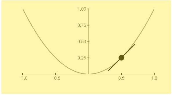
First, we plot the curve on the xy plane and then locate ourselves on the curve at some value of x, say, x = 0.5. At that point, the curve has a slope. One way to find the slope of a curve is to draw a tangent to the curve at the point of interest. The tangent is a straight line. Imagine walking a smidgen along the straight line. You would be at a new location, where the x-coordinate has changed by an infinitesimal amount (Δx; read that as “delta x”) and the y-coordinate has also changed by a corresponding infinitesimal amount (Δy). The slope is . (If you think of climbing stairs, then the slope of the stairs is given by the rise divided by the run, where the rise is Δy, or how much you go up vertically with each step, and the run is Δx, the amount you move horizontally with each step.) Of course, when you do this in our example, you have moved along the tangent to the curve, not along the curve itself. So, the slope really pertains to the tangent and not the curve. However, if the change in the x-direction, Δx, approaches zero, then the slope of the tangent line gets closer and closer to the slope of the curve at the point of interest, until the two become the same when Δx = 0. But how do you calculate the slope when the denominator in is zero? That’s where calculus steps in. Differential calculus is a branch of calculus that lets us calculate the slope of a continuous function (one that has no cusps, breaks, or discontinuities). It lets you analytically derive the slope in the limit ∆x → 0 (read that as “delta-x tends to zero”), meaning the step you take in the x-direction becomes vanishingly small, approaching zero. This slope is called the derivative of a function.

Ananthaswamy then asks “But what do we do when the function involves multiple variables?”:

Well, there’s an entire field of so-called multi-variable, or multi-variate, calculus. And while it can be daunting to confront multi-variate calculus in its entirety, we can appreciate the central role it plays in machine learning by focusing on some simple ideas. Imagine you are standing at some point on the surface of an elliptic paraboloid, z = x2 + y2. To figure out the direction of steepest descent, we must be concerned about two directions, given that we have two variables. Following Thompson’s exhortation to state things in simple ways, we know that moving along the surface means a small change in the value of the variable z. So, our job is to calculate ; or a “tiny change in z divided by a tiny change in x” and a “tiny change in z divided by a tiny change in y,” respectively. In calculus- speak, we are taking the partial derivative of z with respect to x, and the partial derivative of z with respect to y … For a multi-dimensional or high-dimensional function (meaning, a function of many variables), the gradient is given by a vector. The components of the vector are partial derivatives of that function with respect to each of the variables. Our analysis has also connected the dots between two important concepts: functions on the one hand and vectors on the other. Keep this in mind. These seemingly disparate fields of mathematics—vectors, matrices, linear algebra, calculus, probability and statistics, and optimization theory (we have yet to touch upon the latter two)—will all come together as we make sense of why machines learn.

Anansaswamy then introduces us to the role of estimates in machine learning:

Recall from our previous discussion that the gradient is simply a vector in which each element is the partial derivative of the mean squared error, J, with respect to each weight. Each element of this vector will be an analytic expression that can be calculated using the rules of calculus. Once you have the expressions, you just plug in the current values for the weights, and you get the gradient, which you can then use to calculate the new weights. The problem: You need calculus, and while our gradient has only three elements, in practice, it can have elements that number in the tens, hundreds, thousands, or even more. Widrow and Hoff were after something simpler … Instead of calculating the entire gradient, they decided to calculate only an estimate of it. The estimate would be based on just one data point. It didn’t involve calculating the expectation value of the error squared. Rather, they were simply estimating it. But estimating a statistical parameter based on just one sample is usually anathema. Even so, Widrow and Hoff went with it … This is simple algebra. Basically, for each input, you calculate the error and use that to update the weights. Widrow and Hoff were aware that their method was extremely approximate. And yet, the algorithm gets you close to the minimum of the function. It came to be called the least mean squares (LMS) algorithm. In a video Widrow uploaded in 2012, to explain the algorithm, he credited one of his graduate students for naming the algorithm, but he doesn’t remember the student’s name. He also said, “I hope that all this algebra didn’t create too much mystery. It’s all quite simple once you get used to it. But unless you see the algebra, you would never believe that these algorithms could actually work. Funny thing is they do. The LMS algorithm is used in adaptive filters. These are digital filters that are trainable…Every modem in the world uses some form of the LMS algorithm. So, this is the most widely used adaptive algorithm on the planet.” Not only would the LMS algorithm find uses in signal processing, but it would also become the first algorithm for training an artificial neuron that used an approximation of the method of steepest descent. To put this into context: Every deep neural network today—with millions, billions, possibly trillions of weights—uses some form of gradient descent for training. It would be a long road from the LMS algorithm to the modern algorithms that power AI, but Widrow and Hoff had laid one of the first paving stones. Having verified that the algorithm worked, the two had as their next step the building of a single adaptive neuron—an actual hardware neuron. But it was late afternoon. The Stanford supply room was closed for the weekend. “Well, we weren’t going to wait,” Widrow told me. The next morning, the two of them walked over to Zack Electronics, in downtown Palo Alto, and bought all the parts they needed. They then went over to Hoff’s apartment and worked all of Saturday and most of Sunday morning. By Sunday afternoon, they had it working. “Monday morning, I had it sitting on my desk,” Widrow recalled. “I could invite people in and show them a machine that learns. We called it ADALINE—‘adaptive linear neuron.’ It was…not an adaptive filter, but an adaptive neuron that learned to be a good neuron.” What ADALINE does, using the LMS algorithm, is to separate an input space (say, the 16-dimensional space defined by 4×4, or 16, pixels) into two regions. In one region are 16-dimensional vectors, or points that represent, say, the letter “T.” In another region are vectors that represent the letter “J.” Widrow and Hoff chose 4×4 pixels to represent letters, as this was big enough to clearly show different letters, but small enough to work with, given that they had to adjust the weights by hand (using knobs). Anything larger, and they’d have spent most of their time twiddling those knobs. Again, here are the letters “T” and “J” in 4×4-pixel space:

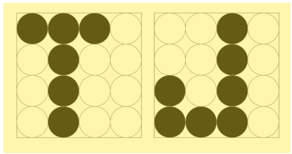
So, each letter is represented by 16 binary digits, each of which can be either 0 or 1. If you were to imagine plotting these letters as points in a 16D space, then “J” would be a point (vector) in one part of the coordinate space, and “T” in another. The LMS algorithm helps ADALINE find the weights that represent the linearly separating hyperplane—in this case, a plane in fifteen dimensions—that divides the input space into two. It’s exactly what Rosenblatt’s perceptron does, using a different algorithm.

By the way, here's a nice video of Widrow himself showing how a machine can teach itself pattern recognition.

Back to Ananthaswamy:

While the perceptron convergence proof … showed clearly why the perceptron finds the linearly separating hyperplane, if one exists, it wasn’t exactly clear why the rough-and-ready LMS algorithm worked. Years later, Widrow was waiting for a flight in Newark, New Jersey. He had a United Airlines ticket. “Those days, your ticket was in a jacket. And there was some blank space on it. So, I sat down and started doing some algebra and said, ‘Goddamn, this thing is an unbiased estimate.’” He was able to show that the LMS algorithm, if you took extremely small steps, got you to the answer: the optimal value for the weights of either the neuron or the adaptive filter. “By making the steps small, having a lot of them, we are getting an averaging effect that takes you down to the bottom of the bowl,” Widrow said. Hoff finished his Ph.D. with Widrow and was doing his postdoctoral studies when a small Silicon Valley start-up came calling. Widrow told him to take the job. It was sound advice: The start-up was Intel. Hoff went on to become one of the key people behind the development of the company’s first general-purpose microprocessor, the Intel 4004 … Other algorithms, also foundational, were being invented … And these non-neural network approaches were establishing the governing principles for machines that learn based on, for example, probability and statistics, our next waystation.

In the next essay in this series, we’ll explore the role of probability in machine learning.